概述

一般方法

截屏2023-02-01 01.19.04

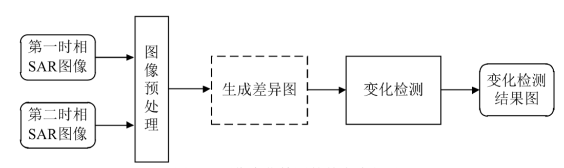
第一步,在进行变化检测之前需要对两幅图像进行几何校正、辐射校正以及去噪
等预处理操作。

  • 几何校正是指SAR成像过程中,由于传感器姿态、地球旋转等条件的影响会使原始图像上地物的特征与其对应的地面地物的特征发生几何畸变, 所以在变化检测之前需要对图像执行几何校正操作。
  • 辐射校正是指图像在获取、传输过程中会发生辐射失真的现象,因此在图像预处理的过程中有必要进行辐射校正。
  • 图像去噪是指SAR传感器在成像过程中会被相干斑噪声干扰,导致获取的图像不能准 确而真实的反映出地物信息,故在SAR图像变化检测之前有必要对相干斑噪声进行滤除。

第二步,生成差异图是指对两幅SAR图像进行某种操作从而生成为一幅图像 的过程。值得注意的是生成差异图这一步骤在SAR图像变化检测中并不是不可或缺的(该步骤表示为虚线框),经过近年来的研究可知,变化信息可以通过直接对预处理后的图像进行操作来获得。

第三步,采用变化检测算法对差异图或预处理之后的图像以有监督或无监督的方式进行分类,进而得到变化检测结果图

评价指标

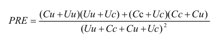
假设,在变化检测结果图中,实际发生变化但检测为未变化的像素点数为Cu, 实际未发生变化但检测为变化的像素点数为Uc,实际未发生变化且检测为未变化的像素点数为Uu,实际发生变化且检测为变化的像素点数为Cc

漏检数False Negatives,FN = Cu

错检数(False Positives,FP = Uc

总错误数(Overall Errors, OE = FN+FP

正确检测率(Percentage Correct Classification,PCC = (Uu+Cc)/(Uu+Cc+Cu+Uc)

Kappa系数Kappa Coefficient,KC = (PCC - PRE)/(1-PRE)

其中

截屏2023-02-01 01.34.08

目前存在的问题

SAR图像存在斑点噪声

训练样本有限

获得的伪标签通常存在误差

网络上的固有问题

深度学习方法(至2020年):https://blog.csdn.net/qq_39932172/article/details/114452418

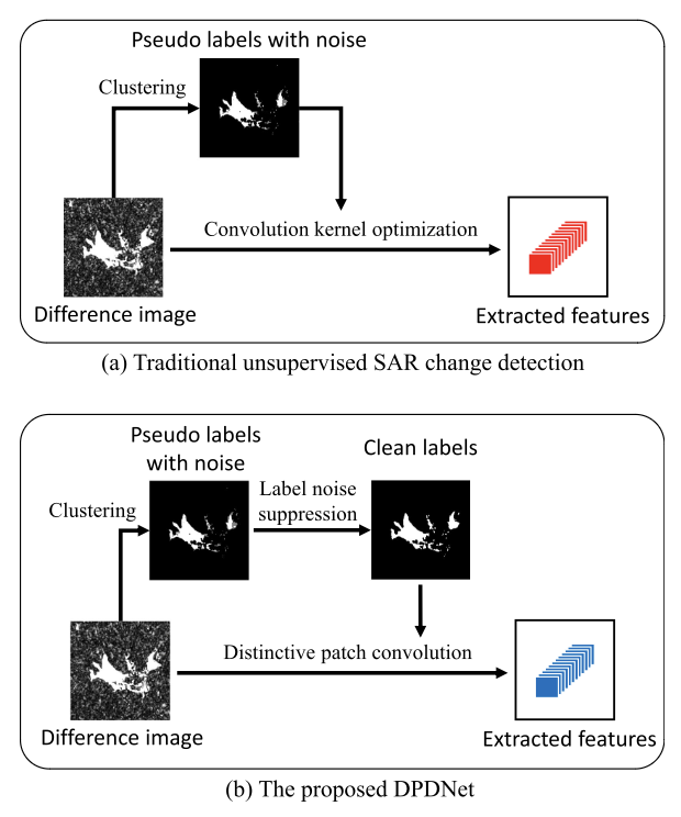
基于双路径去噪网络的SAR图像变化检测 2021

截屏2023-02-02 00.22.43

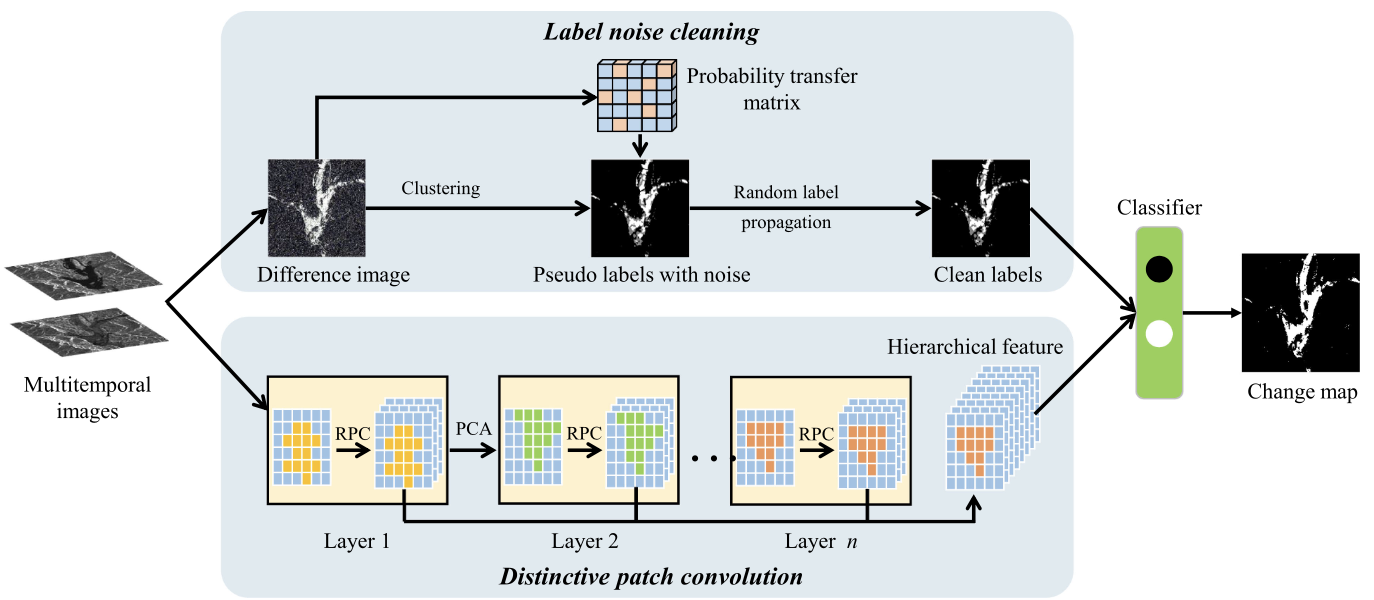
一个分支采用随机标签传播来消除预分类中产生的标签噪声。另一个分支是通过叠加多个卷积层来提取浅层和深层特征。最后,将清洁标签和堆叠特征输入分类器,计算最终的变化检测结果

解决的问题

1)获得的伪标签通常存在误差。

DPDNet的一个分支使用随机标签传播来清除标签噪声。此外,DPDNet的另一个分支用于提取浅层特征和深层特征,然后将它们组合在一起进行分层特征表示。

截屏2023-02-02 00.21.29

2)基于深度学习的方法在训练阶段非常耗时。缺乏大量可靠样本。

主要贡献

  • 首次尝试同时解决散斑噪声和标签噪声的问题。以往的工作主要集中在散斑噪声方面。然而,标签噪声问题不利于变化检测的性能。所提出的DPDNet可以同时缓解两种噪声,并生成更精确的变化图。
  • 提出了一种新的独特的补丁卷积(DPConv),它简化了网络结构,加快了训练阶段。从原始图像中提取的patch被用作卷积核,因此参数优化不需要太多的训练样本。

基于层注意容噪网络的SAR图像变化检测2022

提出了一种基于层注意的噪声容忍网络, LANT-Net,它互连卷积层并且对噪声标签不太敏感。

截屏2023-02-03 00.03.34

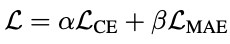
设计了一个用于变化检测的层注意模块,它自适应地对来自不同层的特征进行加权。此外,设计了一个可以有效抑制噪声标签影响的噪声容忍损失函数。它结合了交叉熵 (CE) 损失和平均绝对误差 (MAE)。因此,网络对噪声标签不太敏感并且收敛速度快。

解决的问题

  1. 卷积层之间的特征交互。现有的自注意力增强 CNN 通常在卷积层之后包含一个注意力块,它忽略了多层卷积之间的相互作用。鉴于此,探索卷积层之间的信息流至关重要。
  2. 伪标签中涉及的错误。现有的无监督变化检测方法通常使用聚类来生成具有高训练置信度的伪标签。然而,错误参与伪标签限制网络优化。因此,为无监督变化检测任务建立一个噪声容忍模型是至关重要的。

主要贡献

  • 提出了一个层注意模块,它利用了多层卷积的相关性。来自不同卷积层的特征相互协作,有效地提高了网络的表示能力。

  • 引入了噪声容忍损失函数来减轻伪标记样本中噪声标签的影响。它使模型对噪声标签不那么敏感,收敛速度快。

  • 代码开源

技术细节

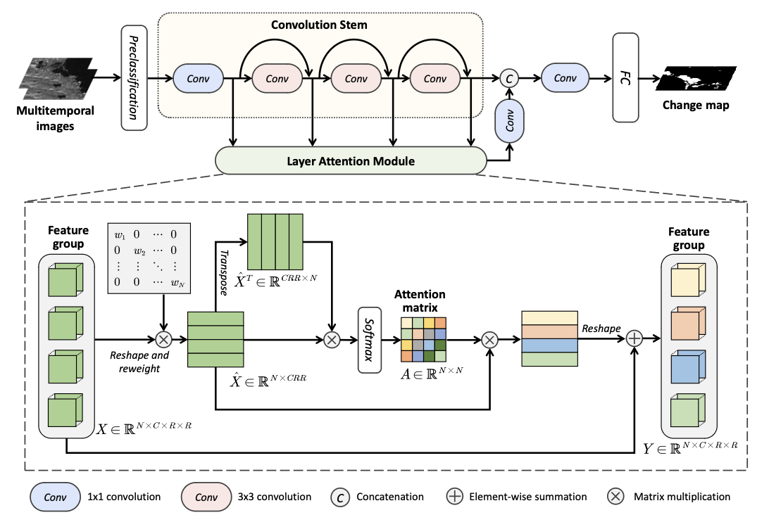
LANTNet 包括三个组件:预分类模块、卷积干和层注意模块。

预分类使用ratio operator 和 the hierarchical Fuzzy C-Means。将I1、I2、差异图像拼接成3 × R × R,作为输入

卷积干由四个卷积层组成,第一个1*1通道数16,然后三个3*3通道数32,中途生成的特征组合起来,并送入层注意力模块。

层注意模块

输入X,维度N*C*R*R,N为4(卷积数),C在代码中为32,reshape为N*CRR

随后,用矩阵乘法将对角矩阵W与特征图相乘,来加权来自不同层的特征。(W被初始化为单位矩阵)结果记为X^
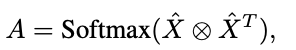
然后计算注意力矩阵A。⊗表示矩阵乘法

截屏2023-02-03 00.33.04

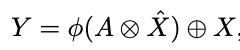
将X^乘以A,reshape为N*C*R*R。与X相加,得到Y。其中φ表示reshape操作。

截屏2023-02-03 00.35.54

最后通过1*1卷积,FC层,Softmax回归,得到结果。

损失函数

{(xi, yi)|1 ≤ i ≤ m} , 其中xi是输入图像补丁,yi是与xi相关的标签,m是样本总数

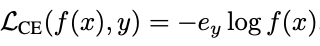
平均绝对误差 (MAE) Loss,其中f(·)表示网络,ey是one-hot向量

截屏2023-02-03 00.42.03

交叉熵 (CE) Loss

截屏2023-02-03 00.42.07

结合起来,α设置为0.1,β设置为0.9

截屏2023-02-03 00.42.13

数据集和评价指标

第一个数据集为巢湖数据集,大小为384 × 384像素。这颗卫星分别于2020年5月和7月在中国被Sentinel-1传感器捕获。第二个数据集是渥太华数据集,大小为290 × 350像素,分别由Radarsat传感器于1997年5月和8月获取。渥太华数据集显示了受洪水影响的变化地区。第三个数据集是苏兹伯格数据集,由欧洲航天局的Envisat卫星于2011年3月11日和16日捕获。这两张照片都显示了海啸引起的冰架破裂

采用假阳性(FP)、假阴性(FN)、总体误差(OE)、正确分类率(PCC)和Kappa系数(KC)五个常用的评价指标对变化检测性能进行评价。

代码实现

https://github.com/summitgao/LANTNet

1
2
3
4
5
6
7
8
9
10
11
12
13
14
15
16
17
18
19
20
21
22
23
24
25
import numpy as np
import skimage
from skimage import io, measure
import random
import scipy.io as sio
import matplotlib
import matplotlib.pyplot as plt
from preclassify import del2, srad, dicomp, FCM, hcluster
import torch
import torchvision
from torchvision import transforms
import torch.nn as nn
import torch.optim as optim
import torch.nn.functional as F
import cv2
from collections import Counter


im1_path = 'Farmland_1.bmp'
im2_path = 'Farmland_2.bmp'
imgt_path = 'Farmland_gt.bmp'


# important parameter
patch_size = 7

定义相关函数

1
2
3
4
5
6
7
8
9
10
11
12
13
14
15
16
17
18
19
20
21
22
23
24
25
26
27
28
29
30
31
32
33
34
35
36
37
38
39
40
41
42
43
44
45
46
47
48
49
50
51
52
53
54
55
56
57
58
59
60
61
62
63
64
65
66
67
68
69
70
71
72
73
74
75
76
77
78
79
80
81
82
83
84
85
86
87
88
89
90
91
92
93
94
95
96
97
98
99
100
101
102
103
104
105
106
107
108
109
110
111
112
113
114
115
116
117
118
119
120
121
122
123
124
125
126
127
128
129
130
131
132
133
134
135
136
137
138
def image_normalize(data):
import math
_mean = np.mean(data)
_std = np.std(data)
npixel = np.size(data) * 1.0
min_stddev = 1.0 / math.sqrt(npixel)
return (data - _mean) / max(_std, min_stddev)

# r是margin
def image_padding(data,r):
if len(data.shape)==3: # 三维,第三个维度不需要
data_new=np.lib.pad(data,((r,r),(r,r),(0,0)),'constant',constant_values=0)
return data_new
if len(data.shape)==2: # 二维
data_new=np.lib.pad(data,r,'constant',constant_values=0)
return data_new
#生成自然数数组并打乱
def arr(length):
arr=np.arange(length-1)
#print(arr)
random.shuffle(arr)
#print(arr)
return arr


# 在每个像素周围提取 patch ,然后创建成符合 pytorch 处理的格式
def createTrainingCubes(X, y, patch_size):
# 给 X 做 padding
margin = int((patch_size - 1) / 2)
zeroPaddedX = image_padding(X, margin)
# 把类别 uncertainty 的像素忽略
ele_num1 = np.sum(y==1)
ele_num2 = np.sum(y==2) # 标记为不变和变的个数
print(X.shape[2])
patchesData_1 = np.zeros( (ele_num1, patch_size, patch_size, X.shape[2]) ) # 不变,四维
patchesLabels_1 = np.zeros(ele_num1)

patchesData_2 = np.zeros((ele_num2, patch_size, patch_size, X.shape[2])) #变
patchesLabels_2 = np.zeros(ele_num2)

patchIndex_1 = 0 #记录是第几个不变的patch
patchIndex_2 = 0
for r in range(margin, zeroPaddedX.shape[0] - margin):
for c in range(margin, zeroPaddedX.shape[1] - margin):
# remove uncertainty pixels
if y[r-margin, c-margin] == 1 : # 不变
patch_1 = zeroPaddedX[r - margin:r + margin + 1, c - margin:c + margin + 1] #(r,c)对应的patch,三维
patchesData_1[patchIndex_1, :, :, :] = patch_1
patchesLabels_1[patchIndex_1] = y[r-margin, c-margin] # 1
patchIndex_1 = patchIndex_1 + 1
elif y[r-margin, c-margin] == 2 : # 变
patch_2 = zeroPaddedX[r - margin:r + margin + 1, c - margin:c + margin + 1]
patchesData_2[patchIndex_2, :, :, :] = patch_2
patchesLabels_2[patchIndex_2] = y[r-margin, c-margin] # 2
patchIndex_2 = patchIndex_2 + 1
patchesLabels_1 = patchesLabels_1-1
patchesLabels_2 = patchesLabels_2-1

#调用arr函数打乱数组
arr_1=arr(len(patchesData_1))
arr_2=arr(len(patchesData_2))

train_len=8000 #设置训练集样本数
pdata=np.zeros((train_len, patch_size, patch_size, X.shape[2])) # 8000*7*7*3
plabels = np.zeros(train_len)

for i in range(7000): # 不变的各个patch
pdata[i,:,:,:]=patchesData_1[arr_1[i],:,:,:]
plabels[i]=patchesLabels_1[arr_1[i]]
for j in range(7000,train_len):
pdata[j,:,:,:]=patchesData_2[arr_2[j-7000],:,:,:]
plabels[j]=patchesLabels_2[arr_2[j-7000]]

return pdata, plabels # 得到数据(len*p*p*3)和标签


def createTestingCubes(X, patch_size):
# 给 X 做 padding
margin = int((patch_size - 1) / 2)
zeroPaddedX = image_padding(X, margin)
patchesData = np.zeros( (X.shape[0]*X.shape[1], patch_size, patch_size, X.shape[2]) )
patchIndex = 0
for r in range(margin, zeroPaddedX.shape[0] - margin):
for c in range(margin, zeroPaddedX.shape[1] - margin):
patch = zeroPaddedX[r - margin:r + margin + 1, c - margin:c + margin + 1]
patchesData[patchIndex, :, :, :] = patch
patchIndex = patchIndex + 1
return patchesData


# Inputs: gtImg = ground truth image
# tstImg = change map
# Outputs: FA = False alarms
# MA = Missed alarms
# OE = Overall error
# PCC = Overall accuracy
def evaluate(gtImg, tstImg):
gtImg[np.where(gtImg>128)] = 255
gtImg[np.where(gtImg<128)] = 0
tstImg[np.where(tstImg>128)] = 255
tstImg[np.where(tstImg<128)] = 0
print(gtImg.shape)
[ylen, xlen] = gtImg.shape
FA = 0
MA = 0
label_0 = np.sum(gtImg==0)
label_1 = np.sum(gtImg==255)
print(label_0)
print(label_1)

for j in range(0,ylen):
for i in range(0,xlen):
if gtImg[j,i]==0 and tstImg[j,i]!=0 :
FA = FA+1
if gtImg[j,i]!=0 and tstImg[j,i]==0 :
MA = MA+1

OE = FA+MA
PCC = 1-OE/(ylen*xlen)
PRE=((label_1+FA-MA)*label_1+(label_0+MA-FA)*label_0)/((ylen*xlen)*(ylen*xlen))
KC=(PCC-PRE)/(1-PRE)
print(' Change detection results ==>')
print(' ... ... FP: ', FA)
print(' ... ... FN: ', MA)
print(' ... ... OE: ', OE)
print(' ... ... PCC: ', format(PCC*100, '.2f'))
print(' ... ... KC: ', format(KC*100, '.2f'))


def postprocess(res):
res_new = res
res = measure.label(res, connectivity=2)
num = res.max()
for i in range(1, num+1):
idy, idx = np.where(res==i)
if len(idy) <= 20:
res_new[idy, idx] = 0
return res_new

得到训练和测试数据

1
2
3
4
5
6
7
8
9
10
11
12
13
14
15
16
17
18
19
20
21
22
23
24
25
26
27
28
29
30
31
32
33
34
35
36
37
38
39
40
# read image, and then tranform to float32
# 读取Sulzberger
im1 = io.imread(im1_path)[:,:,0].astype(np.float32)
im2 = io.imread(im2_path)[:,:,0].astype(np.float32)
from PIL import Image
im_gt = Image.open(imgt_path)
im_gt = np.array(im_gt) # 转换为数组
np.unique(im_gt) # 去重 ,并由小到大排序
print(im1.shape)

im_di = dicomp(im1, im2) # 得到差异图
ylen, xlen = im_di.shape
pix_vec = im_di.reshape([ylen*xlen, 1])


# 分层FCM聚类
# 在预分类图中,
# 大概率不变的像素标记为1
# 大概率被改变的像素标记为2
# 不确定像素标记为1.5
preclassify_lab = hcluster(pix_vec, im_di) # 291*306,层次聚类
print('... ... hiearchical clustering finished !!!')


mdata = np.zeros([im1.shape[0], im1.shape[1], 3], dtype=np.float32)
mdata[:,:,0] = im1
mdata[:,:,1] = im2
mdata[:,:,2] = im_di # 输入的三个通道,分别为图1、图2、得到的差异图

mlabel = preclassify_lab # 聚类得到的lable(无监督)

x_train, y_train = createTrainingCubes(mdata, mlabel, patch_size) #(8000,7,7,3)
x_train = x_train.transpose(0, 3, 1, 2) # 8000,3,7,7
print('... x train shape: ', x_train.shape)
print('... y train shape: ', y_train.shape)


x_test = createTestingCubes(mdata, patch_size)
x_test = x_test.transpose(0, 3, 1, 2)
print('... x test shape: ', x_test.shape)

得到train_loader

1
2
3
4
5
6
7
8
9
10
11
12
13
14
15
16
17
18
19
20
21
""" Training dataset"""
class TrainDS(torch.utils.data.Dataset):
def __init__(self):
self.len = x_train.shape[0] # 8000
self.x_data = torch.FloatTensor(x_train)
self.y_data = torch.LongTensor(y_train)
def __getitem__(self, index):
# 根据索引返回数据和对应的标签

#x=torch.FloatTensor(data_rotate(self.x_data[index].cpu().numpy()))
#y=torch.FloatTensor(gasuss_noise(self.y_data[index]))
#x=torch.FloatTensor(datarotate(self.x_data[index]))
#return x,self.y_data[index]
return self.x_data[index], self.y_data[index]
def __len__(self):
# 返回文件数据的数目
return self.len

# 创建 trainloader 和 testloader
trainset = TrainDS()
train_loader = torch.utils.data.DataLoader(dataset=trainset, batch_size=128, shuffle=True, num_workers=2)

层注意力

1
2
3
4
5
6
7
8
9
10
11
12
13
14
15
16
17
18
19
20
21
22
23
24
25
26
27
28
29
30
31
32
33
34
35
36
37
38
39
# 层注意力
class LayerAttention(nn.Module):
def __init__(self, N): # N = 4
super(LayerAttention, self).__init__()
self.N = N
self.weight = nn.Parameter(torch.eye(self.N,requires_grad=True)) # 对角阵
self.softmax = nn.Softmax(dim=-1)

def forward(self,x):
# B x N x C x H x W
B, N, C, H, W = x.size()
group_mat = x.view(B, N, -1) # B*N*CHW 128*4*1568(32*7*7)

# 只更新权重矩阵对角线上的元素
gradient_mask = torch.zeros(4, 4)
gradient_mask[0, 0] = 1.0
gradient_mask[1, 1] = 1.0
gradient_mask[2, 2] = 1.0
gradient_mask[3, 3] = 1.0
device = torch.device('cuda:0')
gradient_mask = gradient_mask.to(device) # 将tensor转移到cuda上,否则报错Expected all tensors to be on the same device(but cpu和cuda:0)
self.weight.register_hook(lambda grad: grad.mul_(gradient_mask))

weight = self.weight.unsqueeze(0).repeat([B,1,1])
reweight = torch.bmm(weight, group_mat) # 矩阵乘法
# 进行转置
reweight_trans = reweight.permute(0, 2, 1)

weight_tmp = torch.bmm(reweight,reweight_trans)
weight_tmp = torch.max(weight_tmp, -1, keepdim=True)[0].expand_as(weight_tmp)-weight_tmp # 让原矩阵的每一行最大值减去相应行的数
attention_weight = self.softmax(weight_tmp)

out = torch.bmm(attention_weight,reweight)
out = out.view(B, N, C, H, W)

out = out + x
out = out.view(B, -1, H, W)

return out

Loss

1
2
3
4
5
6
7
8
9
10
11
12
13
14
15
16
17
18
19
20
# 噪声鲁棒的损失函数
class Loss(torch.nn.Module):
def __init__(self, alpha=0.1, beta=0.9, classes=2):
super(Loss, self).__init__()
self.device = 'cuda' if torch.cuda.is_available() else 'cpu'
self.alpha = alpha
self.beta = beta
self.classes = classes
self.ce = torch.nn.CrossEntropyLoss()

def forward(self, pred, labels):
# CE
ce = self.ce(pred, labels)
# MAE
pred = F.softmax(pred, dim=1)
label_one_hot = torch.nn.functional.one_hot(labels, self.classes).float().to(self.device)
mae = 2 - 2 * (torch.sum(pred * label_one_hot, dim=1)) # 点乘的作用就是取pred的对应类别的那个预测概率
# Loss
loss = self.alpha * ce + self.beta * mae.mean()
return loss

LANTNet网络

1
2
3
4
5
6
7
8
9
10
11
12
13
14
15
16
17
18
19
20
21
22
23
24
25
26
27
28
29
30
31
32
33
34
35
36
37
38
39
40
41
42
43
44
45
46
47
48
49
50
51
52
53
54
55
56
57
58
59
class LANTNet(nn.Module):
def __init__(self):
super(LANTNet, self).__init__()

inchannel = 3
self.conv1 = nn.Conv2d(inchannel, 8, kernel_size=1, stride=1, padding=0, bias=False)
self.bn1 = nn.BatchNorm2d(8)
self.conv1_1 = nn.Conv2d(8, 32, kernel_size=1, stride=1, padding=0, bias=False)
self.bn1_1 = nn.BatchNorm2d(32)


self.conv2_1 = nn.Conv2d(8, 16, kernel_size=3, stride=1, padding=1, bias=True)
self.bn2_1 = nn.BatchNorm2d(16)
self.conv2_11 = nn.Conv2d(16, 32, kernel_size=1, stride=1, padding=0, bias=False)
self.bn2_11 = nn.BatchNorm2d(32)


self.conv2_2 = nn.Conv2d(16, 32, kernel_size=3, stride=1, padding=1, bias=True)
self.bn2_2 = nn.BatchNorm2d(32)
self.conv2_22 = nn.Conv2d(32, 32, kernel_size=1, stride=1, padding=0, bias=False)
self.bn2_22 = nn.BatchNorm2d(32)

self.conv2_3 = nn.Conv2d(32, 32, kernel_size=3, stride=1, padding=1, bias=True)
self.bn2_3 = nn.BatchNorm2d(32)
self.conv2_33 = nn.Conv2d(32, 32, kernel_size=1, stride=1, padding=0, bias=False)
self.bn2_33 = nn.BatchNorm2d(32)


self.lam= LayerAttention(4)

self.conv3 = nn.Conv2d(128, 4, kernel_size=3, stride=1, padding=1, bias=True)
self.bn3 = nn.BatchNorm2d(4)

self.linear1=nn.Linear(196, 10)
self.linear2=nn.Linear(10, 2)

def forward(self, x):

ori_out1 = F.relu(self.bn1(self.conv1(x)))
m1 = F.relu(self.bn1_1(self.conv1_1(ori_out1)))# 统一到32个通道上来(以便进行层注意力计算)

ori_out2 = F.relu(self.bn2_1(self.conv2_1(ori_out1)))
m2 = F.relu(self.bn2_11(self.conv2_11(ori_out2)))# 统一到32个通道上来

ori_out3 = F.relu(self.bn2_2(self.conv2_2(ori_out2)))
m3 = F.relu(self.bn2_22(self.conv2_22(ori_out3)))# 统一到32个通道上来

ori_out4 = F.relu(self.bn2_3(self.conv2_3(ori_out3)))
m4 = F.relu(self.bn2_33(self.conv2_33(ori_out4)))# 统一到32个通道上来

out5 = torch.stack([m1, m2, m3, m4],dim = 1) # 拼接
out5 = self.lam(out5)
out = F.relu(self.bn3(self.conv3(out5)))
out = out.view(out.size(0), -1) # 拉直
#print(out.shape)
out_1 = self.linear1(out)
out = self.linear2(out_1)

return out

训练

1
2
3
4
5
6
7
8
9
10
11
12
13
14
15
16
17
18
19
20
21
22
23
24
25
26
27
# 使用GPU训练,可以在菜单 "代码执行工具" -> "更改运行时类型" 里进行设置
device = torch.device("cuda:0" if torch.cuda.is_available() else "cpu")
istrain = True
# 网络放到GPU上
net =LANTNet().to(device)
criterion = Loss(alpha=0.1, beta=0.9, classes=2).to(device)
optimizer = optim.Adam(net.parameters(), lr=0.001)
net.train()

# 开始训练
total_loss = 0
for epoch in range(60):

for i, (inputs, labels) in enumerate(train_loader):

inputs = inputs.to(device)
labels = labels.to(device)
# 优化器梯度归零
optimizer.zero_grad()
# 正向传播 + 反向传播 + 优化
outputs = net(inputs)
loss = criterion(outputs, labels)
loss.backward()
optimizer.step()
total_loss += loss.item()
print('[Epoch: %d] [loss avg: %.4f] [current loss: %.4f]' %(epoch + 1, total_loss/(epoch+1), loss.item()))
print('Finished Training')

检验

1
2
3
4
5
6
7
8
9
10
11
12
13
14
15
16
17
18
19
20
21
22
23
24
25
26
27
28
# 逐像素预测类别
istrain=False
net.eval()
outputs = np.zeros((ylen, xlen))
glo_fin=torch.Tensor([]).cuda()
dct_fin=torch.Tensor([]).cuda()
for i in range(ylen):
for j in range(xlen):
img_patch = x_test[i*xlen+j, :, :, :]
img_patch = img_patch.reshape(1, img_patch.shape[0], img_patch.shape[1], img_patch.shape[2])
img_patch = torch.FloatTensor(img_patch).to(device)
prediction = net(img_patch)

prediction = np.argmax(prediction.detach().cpu().numpy(), axis=1)
outputs[i, j] = prediction + 1


if (i+1) % 50 == 0:
print('... ... row', i+1, ' handling ... ...')

outputs = outputs-1

plt.imshow(outputs, 'gray')
res = outputs*255
res = postprocess(res)
evaluate(im_gt, res)
plt.imshow(res, 'gray')

基于双域网络的SAR图像变化检测2022

截屏2023-02-03 22.17.06

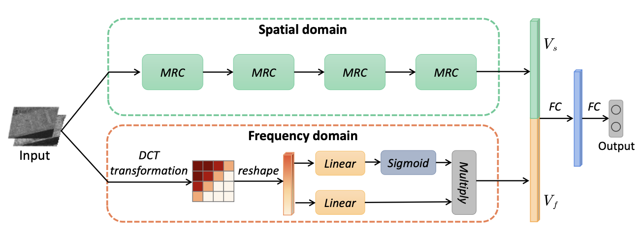
该网络由两个分支组成:一个是用于捕获多区域特征的空间域分支,一个是用于编码DCT系数的频域分支。在空间域分支中,该网络包含四个MRC模块,能够在保留上下文信息的同时强调中心区域特征。在频域分支中,将输入图像补丁通过DCT转换到频域,然后通过“开关”选择DCT系数的关键分量。

解决的问题

  • 现有的方法主要集中在空间域的特征提取上,对频域的特征提取较少关注。

  • 在patch特征分析中,边缘区域可能引入一些噪声特征。

主要贡献

  • 第一个引入DCT域的特征来解决SAR图像变化检测问题。利用了频域和空间两方面的特征。因此,可以有效地抑制散斑噪声
  • 提出了一个MRC模块,它联合强调每个图像补丁的中心区域,同时保留上下文信息。对中心区域特征和上下文信息进行自适应组织以完成分类任务。